Gambling, probability and Bernoulli trials
It is remarkable that a science which began with the consideration of games of chance should have become the most important object of human knowledge.
Pierre-Simon, Marquis de Laplace, Théorie Analytique des Probabilités, 1812
The developments of gambling and probability theory have gone hand in hand throughout history: humans have been playing dice and cards for centuries, humans have then started formalising strategies for wins and losses.
Primitive forms of dice are among the first playthings invented by humanity; card games were likely invented in ancient China in the 9th century. There are references to games in numerous pieces of literature, for instance the “Zara” dice game, from the Middle Ages, is mentioned in Dante Alighieri’s Comedy and other works. The Zara game is very simple: you throw three 6-sided dice at once after choosing a number 3-18 (respectively the minimum and maximum achievable) - because results in the middle of the scale are obtainable with a larger number of dice combinations (you get a 3 with 1-1-1 only, a 18 with 6-6-6 only, a 4 with 1-1-2/1-2-1/2-1-1, a 17 with 6-6-5, 6-5-6, 5-6-6, …, but a 10 or 11 with 27 combos each, out of the 216 possible ones), obviously it’s convenient to bet on them. It does feel like an uninteresting game because of this, but maybe they hadn’t figured it out yet back then! This game is very useful as toy example to teach concepts in probability.
Starting from the 17th century a whole new area of mathematics developed to investigate and formalise the concepts and measurements around chance, odds, wins and losses. Fermat, Pascal, Huygens, Bernoulli, Cardano, de Moivre, Laplace are some of the famous names involved in the founding of this new intellectual endeavour. I’d love to know if the pioneers of probability were also gamblers themselves, but I’m not sure I found reliable information. Either way, it was during their times that playing and gambling took on a whole new level in Europe. It is not uncommon anyway to have people involved in mathematics and forms of gambling or investing to this day - Jim Simons is a brilliant example: a mathematician by background and career with important academic contributions and prizes won, he also worked at the NSA and eventually launched a hedge fund company which made him a billionaire. He’s also been a great philantropist who contributed all his life, monetarily and with time and energy to causes related to the dissemination of scientific education and research, establishing and funding, amongst other nonprofits, “Math for America”.
We’ll give a brief overview of something from the early era of probability theory: Bernoulli trials and the related probability distributions.
The Bernoulli distribution
Let’s consider a binary variable \(X\), that is, one that can take only 2 values, say “1” (usually representing success) with probability \(p\) and “0” (usually representing failure), with probability \(1-p\). Phenomena behaving like this are known as Bernoulli trials - examples are a coin flip or randomly asking people in the street whether they had cereal for breakfast or not.
We can write the probability mass function (the mathematical form of probability for each value) as
\[P (X=x) = p^x(1-p)^{1-x}\]because when \(x=1\) we are left with \(p\) and when \(x=0\) with \(1-p\). This is the Bernoulli distribution.
Expected value (the mean where each value is weighted by its probability) and variance (measuring the spread of values) calculate respectively as
\[\mathbb{E}[X] = \sum_{x \in \{0,1\}} x p^x(1-p)^{1-x} = 0 + 1p(1-p)^0 = p\]and
\[Var[X] = \sum_{x \in \{0,1\}} x^2 p^x(1-p)^{1-x} - p^2 = p - p^2 = p(1-p)\]The Bernoulli responsible for this formalisation was Jakob (there are many famous Bernoullis), son of a pharmacist and brother to Johann. The boys were a bit naughty and disobeyed their father who wanted them to study medicine and theology and did mathemathics instead. We must be very thankful they did as they left us with a huge corpus of important work. Also, Johann’s sons and their sons continued the mathematical dynasty: the Bernoulli family was quite gifted for sure.
More successes and more failures: the Binomial
In this business it’s easy to confuse luck with brains.
Jim Simons [undocumented]
The Bernoulli is a special case of a more general distribution, the Binomial: you have \(k\) successes in a set of \(n\) Bernoulli trials. The probability mass function writes as
\[P(X=k) = {n\choose k} p^k (1-p)^{n-k} \ .\]The first element, \({n}\choose{k}\), quite uncreatively called the “binomial coefficient”, tells you how many ways of creating groups of \(k\) from \(n\) values are there and writes as (with all expansion)
\[\begin{split} {n\choose k} &= \frac{n!}{k!(n-k)!} \\ &= \frac{n(n-1)(n-2) \ldots 1}{(k(k-1)(k-2)\ldots1)((n-k)(n-k-1)(n-k-2)\ldots1)} \\ &= \frac{n(n-1)(n-2) \ldots (n-k+1)}{k (k-1)(k-2)\ldots1} \end{split}\]If you have a bag with 3 balls, named say A, B and C, and want to extract 2 of them (at the same time, that is, with no replacement), you can pick any of 3 different sets: AB, AC, BC, \({3 \choose 2} = \frac{3\cdot2}{2}=3\). If the balls are 4 (A,B,C,D) and you still want a group of 2, you can pick AB, AC, AD, BC, BD, CD, which makes 6 groups or \({4 \choose2} = \frac{4\cdot3}{2\cdot1}\). For group of 3 with 4 balls you can do ABC, ABD, ACD, BCD, \({4\choose 3} = \frac{4\cdot3\cdot2}{3\cdot2\cdot1}\). And so on.
Expected value and variance of the Binomial calculate respectively as \(\mathbb{E}[X] = n p\) and \(Var[X] = n p (1- p)\) (see Wikipedia for the proofs).
Let’s see this with a bit of code.
First the imports and setting up of a pseudo-random number generator in Numpy:
import numpy as np
import matplotlib.pyplot as plt

rng = np.random.default_rng()
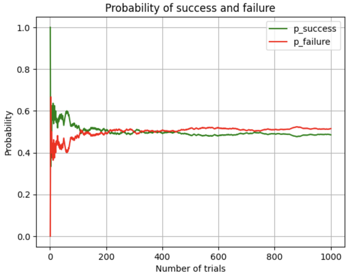
then we simulate 1000 trials of a fair coin flip, that is, one where each face is equiprobable (probability 0.5)
n = 1000    # choose how many trials
trials.append(rng.choice([0,1], size=n))   # numpy.choice will by default use a uniform distr over values
and we count successes and their probability
successes = np.cumsum(trials)
p = successes / np.arange(1, n+1)
which we can plot
plt.plot(np.arange(1, n+1), p, label='p_success', c='g')
plt.plot(np.arange(1, n+1), 1 - p, label='p_failure', c='r')

plt.grid()
plt.legend()

plt.title('Probability of success and failure')
plt.xlabel('Number of trials')
plt.ylabel('Probability')
obtaining these trends:
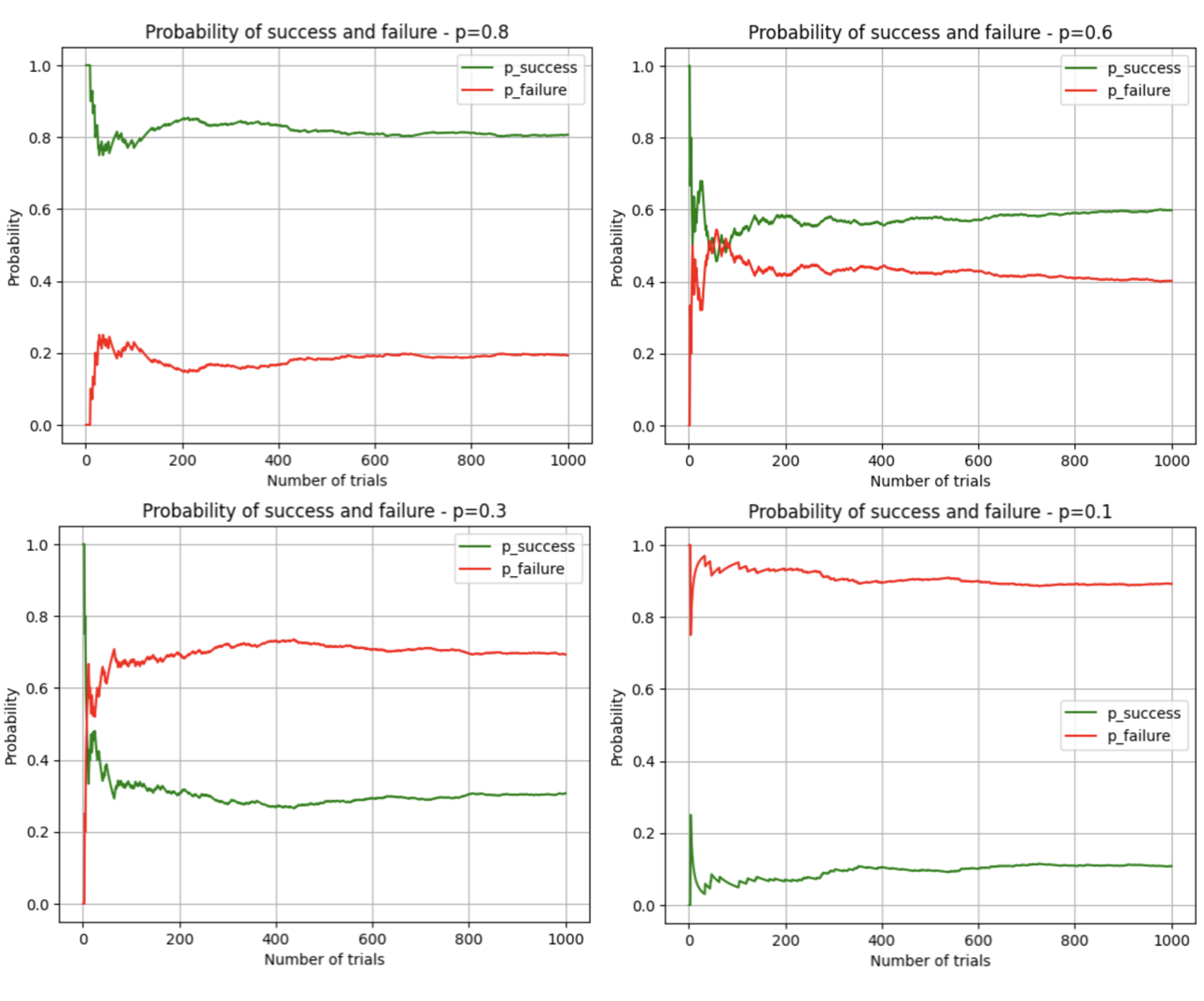
If we vary the probability of success (using arg p in numpy.random.choice), so to represent unfair coins, we get these trends
The Binomial distribution generalises into a Multinomial when possible results are more than two.
Probability theory is full of nice and fun questions.
Good reads
- Probability and Statistics on Encyclopedia Britannica
- J MacDonald, The ancient origins of Dice, JSTOR Daily 2018 - with lots of links to archeology studies
- J Roebke, Putting his money where his math is, Seed Magazine (defunct) 2006, via Web Archive - nice article about J Simons and his passion for maths education
- D T Max, Jim Simons, the numbers King, The New Yorker 2017
- J Eglin, How the 18th-century ‘probability revolution’ fueled the casino gambling craze, The Conversation 2024
- J I García-García, N A Fernández Coronado,E H Arredondo, I A Imilpán Rivera, The Binomial Distribution: Historical Origin and Evolution of Its Problem Situations, Mathematics 2022 (open access)