Entropy, data and Machine Learning

No structure, even an artificial one, enjoys the process of entropy. It is the ultimate fate of everything, and everything resists it.
— P K Dick, Galactic Pot-Healer

That concept of entropy has its roots in thermodynamics where it emerged in the mid of the 19th century as part of that vast intellectual exploit that followed the industrial revolution and was defined from the study of thermal exchange. In an isolated system, which will naturally tend to reach thermal equilibrium, entropy increases as a result - this is the second law of thermodynamics.

L. Boltzmann linked the macroscopic definition of entropy to the microscopic components of the system, rendering entropy into a statistical concept, and J W Gibbs gave further development to the idea, defining it in terms of an aggregation over all possible microstates of a system (the constant is the the Boltzmann constant) as:

\[S = - k_B \sum_i p_i \ln p_i\]

where \(i\) is the index of each microstate and \(p\) its probability. A microstate is a configuration of the microscopic elements of the system (e.g. molecules, in the case of physical matter). Effectively, the entropy is proportional to the expected value of the logarithm of probability.

The popular notion of entropy as a measure of disorder stems from all this: entropy measures (statistically) the ways in which a system can arise from the configuration of its microscopic components.

Rocks crumble, iron rusts, some metals corrode, wood rots, leather disintegrates, paint peels, and people age. All these processes involve the transition from some sort of “orderliness“ to a greater disorder. This transition is expressed in the language of classical thermodynamics by the statement that the entropy of the Universe increases.
— W M Zemansky, R H Dittman, “Heat and Thermodynamics“

Fast-forward a few decades and we have C E Shannon who in 1948, while employed at Bell Labs, wrote the crucial paper “A Mathematical Theory of Communication“, that defined entropy in the realm of Information Theory as a way to measure the level of information in a message. This definition follows the same paradigm:

\[H(X) = - \sum_{x \in A} p(x) \log_2 p(x) = - \mathbb E[\log_2 p(X)] \ ,\]

where \(X\) is a random variable spanning space A the base-2 logarithm is used because of the unit of bits, which can have two states. Note that Shannon used the letter H to refer to entropy, you can read more about the why here. The Shannon entropy is again linked to disorder, or uncertainty: the more similar probabilities are, the higher the entropy.

Let’s make a simple example. Suppose we have a fair coin (one with the same probability of yielding heads or tails, that is, 50%). H would then simply be:

\[H = - \frac{1}{2} \log_2 \frac{1}{2} - \frac{1}{2} \log_2 \frac{1}{2} =- \log_2 \frac{1}{2} = 1\]

In the case of a coin that is maximally unfair on the side of heads (it yields heads every time), we would have H = 0, and the same with a coin maximally unfair on the side of tails. In fact, if p is the probability of yielding heads, then (1-p) would be the probability of yielding tails, and the entropy becomes:

\[H = p \log_2p - (1-p) \log_2(1-p) \ ,\]

which plots as

Graph of the entropy for a coin flip as a function of the (heads) probability p. Graph has been quickly created asking Google to plot the function.

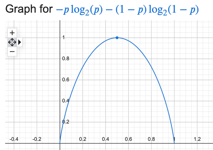
You can see the graph reaches its maximum for the fair coin situation (p=0.5) and is 0 at the extremes: these are the levels of minimum information as the result is directly predictable, with certainty. The fairer the coin, the less predictable the result is, and the higher the informational content. The equiprobable situation is the one with the highest informational content, and highest entropy.

You can extend this reasoning to more complex trials with a higher number of possible states, e.g. a dice which has 6 possible states. In fact, the entropy reaches its maximum value for \(p=1/n\) (a uniform distribution), n being the number of possible states, and that maximum value is the logarithm of n.

Use in Machine Learning

Now why is this relevant to the world of data? Because you can use the entropy as an accessory evaluation metric for the reliability of your ML classifier - it will inform you on how sure your classifier is.

One important note: entropy is not an alien concept to Machine Learning as it is used for instance in tree-based models to decide on each split. But here we are discussing the use of entropy ex post facto, at the inference step.

Suppose you have a probabilistic classifier (one that spits out the inferred class alongside a probability value), examples are tree-based models or logistic regression. Normally in these cases the class inferred with the highest probability is the one furnished in output. But there is information in the probability values! Are they very different, or are they roughly the same, with one of the classes just barely topping the others? In short: is the probability distribution over the classes resembling a uniform or is it far from it?

Intuitively, if for example we had a binary classification (classes A, B) and our inferred result on a new instance were class B with probability 0.8 (which means class A has probability 0.2), we would feel like the classifier is quite sure of its choice. If instead, on another instance, the result were class B with probability 0.52 we wouldn’t feel that convinced. The same extends to multi-class problems.

Knowing that the entropy is maximal and equal to the logarithm of the number of classes in the most confused situation where all classes have the same probability helps us: we can compute the entropy over all our inference instances and analyse results in a statistical fashion. We can for example draw a histogram of the entropy on all the instances, to check how many times the classifier has been quite confused/unsure - maybe these instances are not good enough to keep.

This paper goes further and creates the concept of an “entropy score”, the entropy normalised to its maximum value and then explores an application to the Naive Bayes classifier.

A walkthrough example

I searched for a simple dataset that could illustrate all this well - the requirements were that it had to be suitable for a multi-class classification, ideally with a small number of classes. I could have used a binary classification problem one too, but it would have been a less interesting example, with just two probabilities to calculate the entropy on.

I finally found a 3-class problem in this dataset¹ hosted on Kaggle: diabetes health indicators. It’s free to download. I am only using it as toy example to calculate the entropy so I will not care for the general quality of the classification; for the sake of simplicity I will use a base Random Forest classifier and I will keep track of the probabilities associated to the classified class on a portion of the dataset.

I’ve put all the code in this gist if you’re interested.

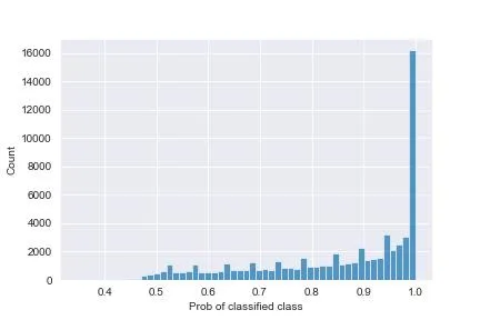
When you plot the histogram of the probabilities of the classified class (the one chosen by the model, which means the one with the highest probabilities amongst the three possible ones) you obtain this plot:

Histogram of the probabilities of the classified class on a test set isolated from the diabetes dataset described in text, which has been used to train a classifier. Plot has been generated using Seaborn.

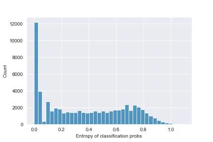
And, correspondingly, the entropies of each classification display this histogram:

Histogram of the entropies of the classification on the same set as in previous picture.

You can see that there’s many items where the probability is exactly 1: the classifier is sure here, and the entropy is 0.

The probabilities are generally quite high, which means this classifier is quite confident in its choices - that’s good. There are, however, a handful of instances in which the max probability is around 0.45 - still higher than a uniform situation (which would see all probabilities at ~0.33), but nevertheless not very good. Here, the entropy is the highest (around 0.99, compare to the logarithm of 3, ~1.58, we would get with a uniform), these are the most confused instances - you may want to discard them in inference and not spit out a classification at all.

To conclude, it can be very useful to do a quick entropy analysis when you are dealing with a classification problem, on top of model evaluation for quality.

References & more reads

• If you want a good traditional book on thermodynamics I can recommend the text by M W Zemansky and R H Dittman, “Heat and Thermodynamics“. I’ve used it during my studies in Physics.
• Wikipedia’s ecosystem on Entropy is quite good, you can learn much about the physics roots and applications.
• C E Shannon, A Mathematical Theory of Communication, Bell System Technical Journal, vol. 27, 1948 (freely available).
• G Tornetta, Entropy Methods for the confidence Assessment of Probabilistic Classification models, Statistica, 2021 (open access)

---

1. Finding a decent dataset for this task proved to be not that trivial, actually. Most toy datasets in circulation are for binary classification problems, or are very small and not interesting from the point of view of classified probabilities (this is the case of the famous Iris dataset, embedded into Scikit-learn, that gave me very all high probabilities for the classified class, which means low entropy). ↩