Dissecting the Gradient descent method

This post has had a good ride. I wrote it first in 2016 but the version here has been modified in Dec. 2023 to accommodate some additions I had somewhere else. Back in the days, it received some praise, so I hope you find it useful.

---

Gradient descent

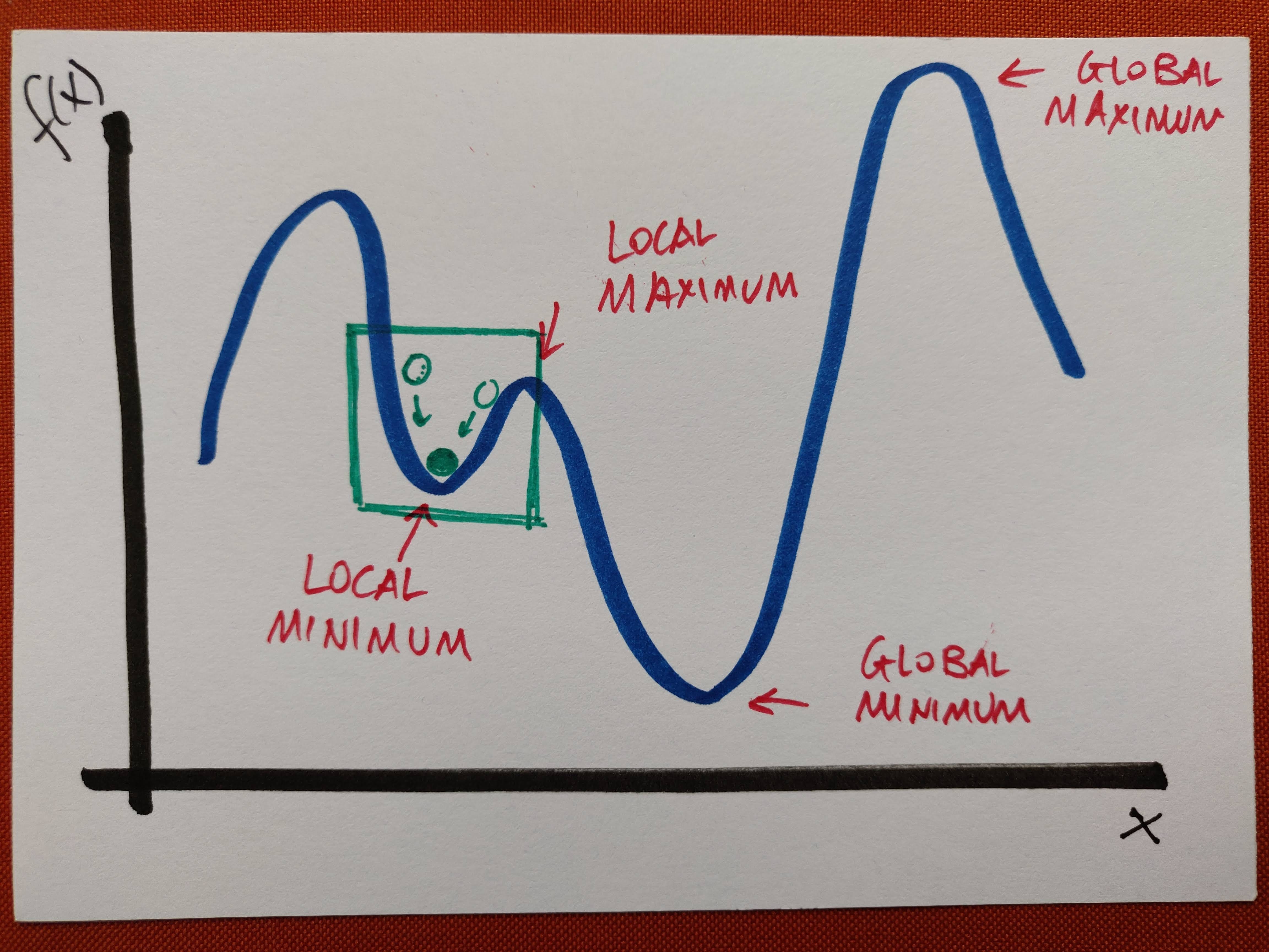
Gradient descent is a general mathematical optimisation method used to find a (local) minimum of a differentiable function. The idea is to follow the direction of the gradient (in 1-dimension, the derivative) as the most economical way to “descend” to a minimum.

Illustration of a 1-dimensional function with local and global minima/maxima. The gradient descent method allows a minimum to be reached in steps, following the direction of the gradient (see green part) - the minimum reached is not guaranteed to be global.

In Machine Learning, this algorithm is used to minimise functions in the form of a sum

\[f(w) = \sum_i^n g_i(w) \ ,\]

which measure the error between the real and the predicted representation of your data.

The errors which arise from the absence of facts are far more numerous and more durable than those which result from unsound reasoning respecting true data.
– Charles Babbage, “On the Economy of Machinery and Manufactures”

For instance, in a linear regression task with ordinary least squares implementation, the function to minimise is the sum of squared residuals between observed and predicted values, over all observations (\(n\) is the number of data points and we are assuming they live in a generic dimensional space, hence \(\bar w\) and \(\bar x\) are treated as vectors):

\[E[\bar w] = \sum_i^n (y_i - \bar w \cdot \bar x_i)^2 \ .\]

If, for the sake of simplicity, we think about this in 1 dimension,

Illustration of a 1-dimensional linear regression: observed data points (n) and fitting line, with residuals highlighted.

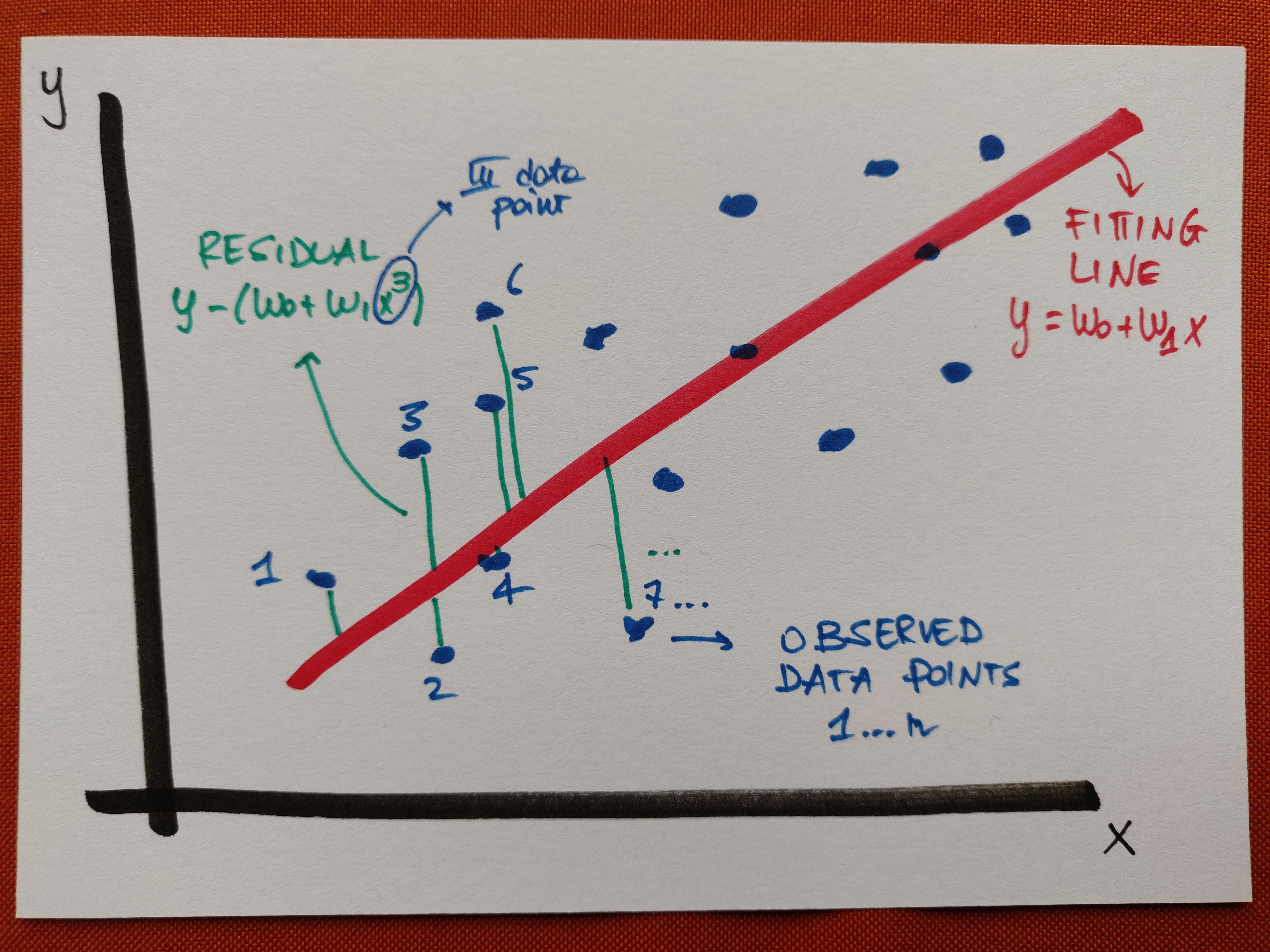
we can easily visualise the residuals, that is, the (vertical) differences between prediction and observation - the goal of a good fit is to minimise the error as the sum of their squares.

In gradient descent, the gradient of the function (or the derivative in the 1-dimensional case) is used to identify the direction of maximum growth of the function, and a “descent” is implemented by updating the parameters iteratively as

\[w := w - \alpha \nabla f(w) = w - \alpha \nabla \left( \sum_i^n g_i(w) \right) \ .\]

The value multiplying the gradient is the learning rate, which is important to choose wisely: if it is too big it might get us past the minimum, trapping us in a zig-zagging motion across it; if it is too small it can slow down the computation because steps taken are tiny. In any case, for the algorithm to terminate, the iteration is set to stop once the difference between the current value of the parameter and the previous iteration’s one falls below a given precision threshold, chosen a priori.

Essentially, the idea is to do what is illustrated in the very first picture above: making the green ball approach the minimum in steps.

What we described is the so-called “standard” gradient descent, which uses all observed data and for that is not the fastest possibility, we will see a speedier modification later.

Standard gradient descent

We will code this in Python, so to start with and follow through here, you need some imports:

import numpy as np
from scipy.spatial.distance import euclidean
from matplotlib import pyplot as plt

Suppose we want to use (standard) gradient descent to minimise a function in the form of a paraboloid (2-dimensional) with minimum in the origin:

\[f(x, y) = x^2 + y^2 \ ,\]

the vector field given by its gradient is graphically represented as per figure (vector lengths are scaled).

The gradient vector field is giving us the direction of growth of the paraboloid, so descending along will lead us towards the desired minimum.

Minimising a 1D parabola

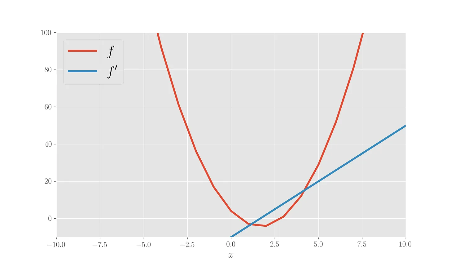
Let’s code a gradient descent towards the minimum of a 1-dimensional parabola starting from \(x=7\) and with a learning rate of \(0.1\). The computation is stopped when the difference between the iteration updates goes below a threshold value set to \(10^{-4}\). Let’s define the parabola and its derivative, plotting both.

# Choose the x points
x = np.array([i for i in range(-1000, 1000)])

# Define the function and its derivative
def f1(x):
    return 3*x**2 - 10*x + 4

def f1_der(x):
    return 6*x - 10

# Plot the functions
plt.ylim(-10,100)
plt.xlim(-10,10)
plt.plot(x, f1(x), label='$f$', lw=3)
plt.plot(x, f1_der(x), label="$f'$", lw=3)
plt.legend(loc=2)
plt.xlabel('$x$')
plt.show()

Then we implement a gradient descent with a chosen learning rate and starting point.

# Running the gradient descent

x0 = 7         # starting point for the descent
alpha = .1     # step size (learning rate)
p = .0001      # chosen precision

former_min = x0
iterative_mins = [former_min]
while True:
    x_min = former_min - alpha * f1_der(former_min)
    iterative_mins.append(x_min)
    if abs(former_min - x_min) <= p:
        break
    else:
        former_min = x_min
        
print('Local min of function is %f' %x_min)

This finds the minimum at \(1.67\). We can plot the iterations:

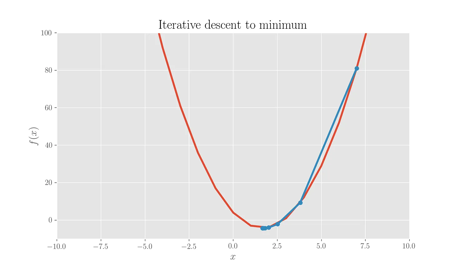
This is pretty satisfactory given that the analytical minimum is exactly at \(10/6=1.67\).

Minimising a 2D parabola

We can do the same but for a paraboloid in 2 dimensions.

# Function and derivative definitions
def f2(x, y):
    return x**2 + y**2

def f2_der(x, y):
    return np.array([2*x, 2*y])

#Running the gradient descent

x0 = 50            # starting point for the descent
y0 = 50            # starting point for the descent
alpha = .1         # step size (learning rate)
p = .0001          # chosen precision

former_min = np.array([x0, y0])
iterative_mins = [former_min]
while True:
    x_min = former_min - alpha * f2_der(former_min[0], former_min[1])
    iterative_mins.append(x_min)
    if abs(former_min[0] - x_min[0]) <= p and abs(former_min[1] - x_min[1]) <= p:
        break
    else:
        former_min = x_min
        
print('Local min of function is', x_min)

which yields a local minimum of \((3.7 \cdot 10^{-4}, 3.7 \cdot 10^{-4})\).

Linear regression

As we said, this method is used in a ordinary least squares calculation for a linear regression to find the line which best fits a bunch of observation points. Let’s “manually” implement it.

Let’s say that we have some experimental data points, and we calculate the objective function for a linear regression (the error):

x = np.array([1, 2, 2.5, 3, 3.5, 4.5, 4.7, 5.2, 6.1, 6.1, 6.8])
y = np.array([1.5, 1, 2, 2, 3.7, 3, 5, 4, 5.8, 5, 5.7])

alpha = 0.001                       # learning rate
p = 0.001

def f(x, w):
    """A line y = wx, to be intended as w0 + w1x (x0 = 1)"""
    return np.dot(x, w)

def diff(a, b):
    return a - b

def squared_diff(a, b):
    return (a - b)**2

def obj_f(w, x, y):
    """The objective function: sum of squared diffs between observations
     and line predictions"""
    return sum([squared_diff(f(np.array([1, x[i]]), w), y[i])
                for i in range(len(x))])

Then we perform a linear regression via minimising it:

def obj_f_der(w, x, y):
    """Gradient of the objective function in the parameters"""
    return sum([np.dot(2 * np.array([1, x[i]]),
                diff(f(np.array([1, x[i]]), w), y[i]))
                for i in range(len(x))])

former_w = np.array([10, 5])    # the chosen starting point for the descent
while True:

    w = former_w - alpha * obj_f_der(former_w, x, y)

    if euclidean(former_w, w) <= p:
        break
    else:
        former_w = w

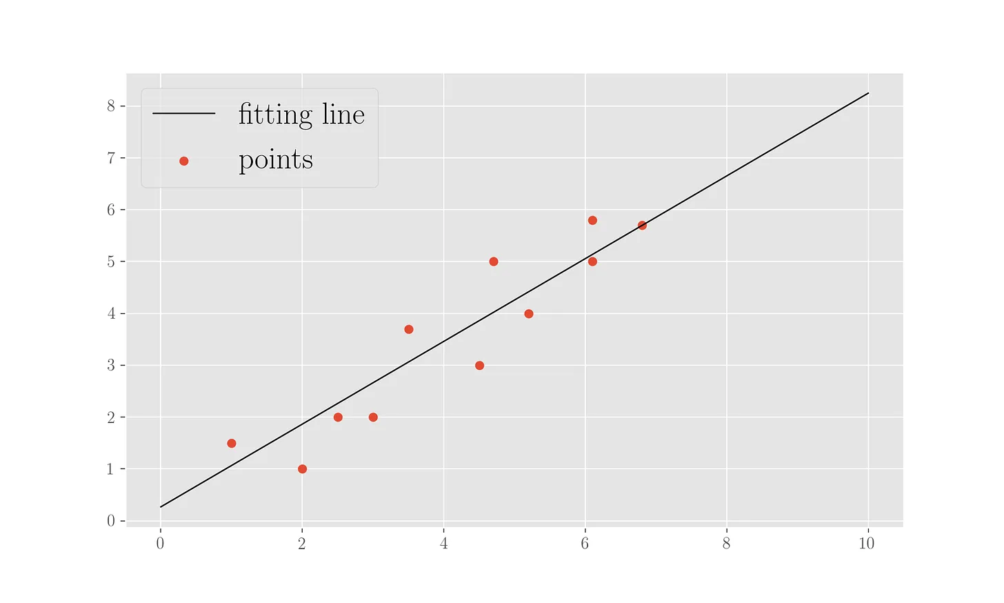
The result of the gradient descent is an intercept \(0.27\) and a slope \(0.80\) for the fitting line. We can plot the line alongside the points:

plt.scatter(x, y, marker='o', label='points')
plt.plot([i for i in range(0,11)], [w[0] + w[1] * i for i in range(0, 11)], label='fitting line', c='k', lw=1)
plt.legend(loc=2)
plt.show();

Stochastic gradient descent

The stochastic version of gradient descent (often shortened as SGD) does not use all points at each iteration to calculate the gradient of the function but picks only one point. The point update of the parameters looks like

\[w := w - \alpha \nabla g_i(w)\]

A for loop across \(i\) passes this rule across all observations in the training set, which has been randomly shuffled (epoch), until the updated parameter does not change by more than a chosen precision.

This is particularly useful for large datasets where the standard updating rule might be too slow to compute due to the sum on all observations (and remember that gradient encompasses derivatives in every dimension). If instead we calculate the gradient only on one point at a time on a randomly shuffled version of the dataset, we obtain a significant save in computation.

Linear regression with SGD

Using the same dataset, same learning rate and same precision as above, we re-implement the descent, this time using the stochastic rule

def obj_f_der_point(w, obs_x, obs_y):
    """Addend of the gradient of the objective function in the parameters"""
    return np.dot(2 * np.array([1, obs_x]), diff(f(np.array([1, obs_x]), w), obs_y))

# Perform a stochastic gradient descent
training_set = [(x[i], y[i]) for i in range(len(x))]

epoch = 1
former_w = np.array([10, 5])      # chosen start for the descent

found = False
max_epochs = 2000
while epoch < max_epochs:
    random.shuffle(training_set)
    for point in training_set:
        w = former_w - alpha * obj_f_der_point(former_w, point[0], point[1])
        if euclidean(former_w, w) <= p:
            break
        else:
            former_w = w
    
    epoch +=1 
    
print(epoch)
print('Found parameters (intercept, slope):', w)

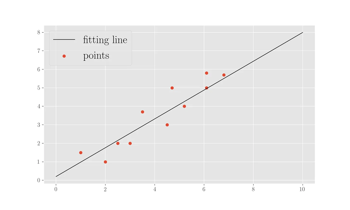
This procedure, which uses 2000 epochs, finds parameters \(0.23\) for the intercept and \(0.80\) for the slope (compare to above where we had \(0.27\) for the intercept). In figure, the points and fitting line for this.

References & read more

• I’ve put the code reported here in a Jupyter notebook
• Some more reading on the scikit-learn documentation, focused on usage

---

I have a newsletter where I post things like this and more, you can subscribe here to get them in your inbox: