
Power laws, beautiful and damned
“She was beautiful - but especially she was without mercy.”
― F. Scott Fitzgerald, “The Beautiful and Damned”
For anyone who worked in science or generally with data, power law distributions are the norm (pun not intended). They are an actual feature of the natural and social world, present in all sorts of phenomena: wealth distributions (Pareto), word frequencies (Zipf), number of node connections in a social network, sales on Amazon…
Newman’s review paper on this topic, “Power laws, Pareto distributions and Zipfs’s law” is a joy to read, you can do so as it’s free and open-access on ArXiv. We will use it to outline why these kinds of distributions are so alluring and deserve thought.
A polemical note (in jest)
Newman says, at the start of the paper, that
Most adult human beings are about 180cm tall.
— M E J Newman, “Power laws, Pareto distributions and Zipfs’s law”
The crux is in the “about”, but this sounds like an exaggeration to me (and that’s not just because I am barely 152cm tall)! Let’s check this statement. I found the SOCR dataset of human height and weight, kindly scraped and organised in a CSV by Kaggle. SOCR stands for “Statistics Online Computational Resource”, it’s a site (with a wonderful early-2000s interface) set up by UCLA for educational purposes. The chosen dataset apparently comes from data simulated based on children’s real heights as measured in a survey. We end up with this distribution of adult heights:
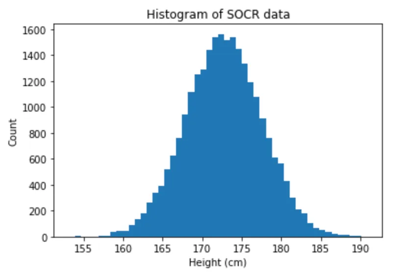
It is very clearly normal, with the mean at 172cm. The third quartile is at 175cm so I’m still right, based on this data, that 180cm is too high to be a representative human height! Note that SOCR doesn’t specify any features of the data, e.g. gender or ethnicity, which may determine differences. Newman is using himself data to make his point though, data from the National Health Examination Survey and he effectively finds a distribution mean around 180cm.
Back to power laws now.
What are power laws
Power laws are relations of the form (A is a constant and \(\alpha\) is a positive number1):
\[f(x) = A x^{-\alpha}\]which, if we apply a logarithm to both sides, become
\[\log f(x) = \log A - \alpha \log x \ .\]This is why they appear linear in a log-log plot, which makes them easier to visualise.
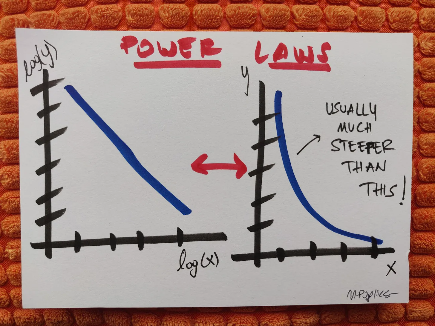
In a probabilistic context, a variable distributed in a power law way is one where there’s very many elements with low values and some with extremely large values, so not only do you see no characteristic “peak”, but you also cannot easily describe the distribution by a simple representative number.
Citing directly from Newman’s paper, where he used genuine data, examples of things distributed in a power-law way are (see figure below):
- Frequencies of words in a text - there are always some very common words (think of articles, prepositions, or words specific to the topic of the text) and very many low-frequency ones.
- Citations to scientific papers published in a given year.
- Traffic to websites - we all know a few sites which are massive, and then most blogs/sites don’t get much traction.
- Bestsellers books sales in a given period: the distribution here is already cutting off the long tail of those books that sell nothing. Note that the same would apply to sales of pretty much everything else.
- Phone calls received by a given set of numbers: the hubs would be your most popular friends, or e.g. utility companies.
- Magnitude of earthquakes - mercifully, just a few are really catastrophic. Note that here the x-axis is linear because earthquakes’ magnitude is already defined as a logarithm.
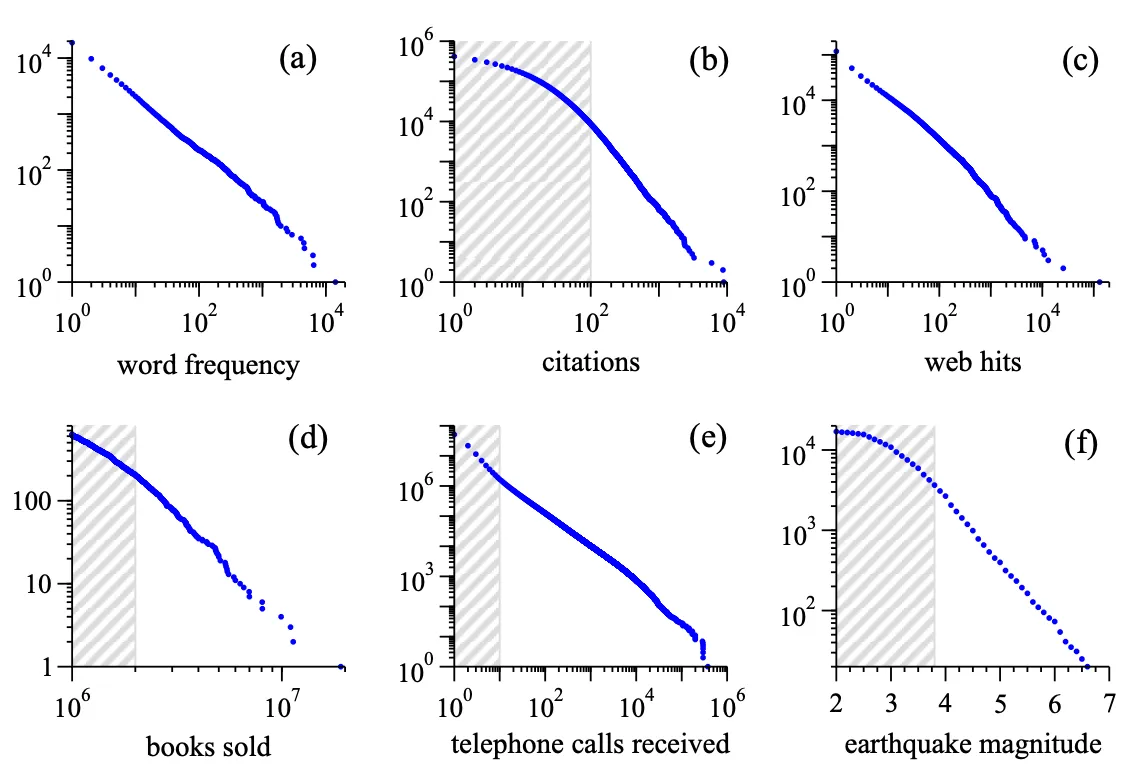
There’s more examples and more details in the paper.
Note that it isn’t completely correct to say that “a lot of phenomena follow a power-law distribution”, because usually it’s only the tail that does. Real-world data distributions can be tricky to analyse, and simply drawing them in log-log is a poor way to ascertain a power-law behaviour, as there can be several other possibilities. However, the power law model works well as a guideline.
A few reasons why power laws are interesting
Scale invariance
Power laws benefit from scale invariance, which means that if x scales by a multiplicative factor, the shape of the function remains the same bar a multiplier:
\[f(Bx) = A B^{-\alpha} x^{-\alpha} = B^{-\alpha} f(x) \ .\]This property is very interesting in areas like the physics of materials and statistical mechanics, where it describes the emergence of phase transitions. It implies the power law relation lacks a typical scale.
As probability density function: expected value
Because \(f(x)\) diverges for \(x=0\) this means that in practical terms as a probability density function
\[p(x) = A x^{-\alpha}\]it must have a minimum value greater than 0. Let’s indicate it with the suffix min.
The expected value calculates then as
\[\begin{align} \mathbb{E}[X] &= \int_{x_{min}}^{\infty} p(x) x \mathrm{d} x \\ &= \int_{x_{min}}^{\infty} A x^{1-a} \mathrm{d} x \\ &= \frac{A}{2-a} x^{2-a} \vert_{x_{min}}^{\infty} \end{align}\]which diverges if \(a <= 2\): power law distributions can have infinite means.
Consequences of this are non trivial. If you have a finite sample of values you can always (obviously) calculate the mean, even when the population is distributed with a power law. But in that case a sample mean may not be in line with the population mean: different samples may lead to very different sample means, because some will be characterised by extremely large values. The mean is not a representative value for the distribution.
Similar reasonings arise with higher momenta, for instance you can calculate that the variance (hence the standard deviation) diverges if \(a <= 3\).
A fat tail
The power law distribution is also known, in jargon, as a “fat-tail”. To be correct though, a fat-tail distribution is one whose tail behaves like a power-law.
If a distribution has a fat-tail it means that the probability of extreme values is quite chunky (compared to e.g. a normal distribution). “Fat-tail” and “heavy-tail” are often used interchangeably, but in reality the first is a subset of the second - a “heavy” tail is one which is chunkier in the tail than an exponential, so decreases more slowly. A “fat” tail is “heavy” but the reverse isn’t always true - an example is the log-normal distribution, chunkier than an exponential but slimmer than a power (decreases faster). In the references you find a link to a very good discussion on Cross Validated on this difference.
To have a reference mental model, a fat tail is fatter than the tail of a normal distribution, where we know that the probability of staying within one/two/three standard deviations of the mean is respectively ~68%/~95%/~99%. In a fat tail, large values can appear with higher chance, making it hard(er) to call them “outliers”.
Because these distributions are so ubiquitous, this matter isn’t just an erudite academic one. The scholar N N Taleb has done much work on the concept of “black swan” (hard to predict, different from the rest and consequential events) and the fact that in fields like economics the blind use of the canonical instruments of descriptive statistics, usually developed for gaussians (e.g. using means to represent a distribution, calculating standard deviations, …), can lead to disaster. He says:
The traditional statisticians approach to thick tails has been to claim to assume a different distribution but keep doing business as usual, using same metrics, tests, and statements of significance. Once we leave the yellow zone, for which statistical techniques were designed (even then), things no longer work as planned.
— N N Taleb, “Statistical consequences of fat tails”
I’m leaving some good stuff in the references. So we need to watch out, when we analyse data.
We’ll likely expand this topic some other posts in this section.
References
- M E J Newman, Power laws, Pareto distributions and Zipfs’s law, Contemporary Physics 46.5 (2005)
- Cross Validated discussion on the difference between a heavy-tail and a fat-tail distribution
- A video excerpt from a talk by N N Taleb on the concept of “Black Swan”
- N N Taleb, Statistical Consequences of Fat Tails: Real world preasymptotics, epistemology, and applications, ArXiv preprint (2020)
-
\(\alpha\) could very well be a negative number too, for a general power-law relation. However, for the sake of the following, we are specialising in relations where the exponent is negative. ↩